Image classification using GoogleNet Convolutional Neural Network on a Raspberry Pi
Convolutional Neural Networks
In machine learning, a convolutional neural network (CNN, or ConvNet) is a class of deep, feed-forward artificial neural networks that has successfully been applied to analyzing visual imagery.
CNNs use relatively little pre-processing compared to other image classification algorithms. This means that the network learns the filters that in traditional algorithms were hand-engineered. This independence from prior knowledge and human effort in feature design is a major advantage.
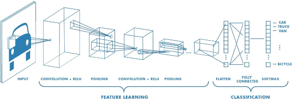
Figure 1: Convolutional Neural Network
Architectrure
A CNN consists of an input and an output layer, as well as multiple hidden layers. The hidden layers of a CNN typically consist of convolutional layers, pooling layers, fully connected layers and normalization layers.
Convolutional:
Convolutional layers apply a convolution operation to the input, passing the result to the next layer. The convolution emulates the response of an individual neuron to visual stimuli.
Each convolutional neuron processes data only for its receptive field. Tiling allows CNNs to tolerate translation of the input image (e.g. translation, rotation, perspective distortion).
Although fully connected feedforward neural networks can be used to learn features as well as classify data, it is not practical to apply this architecture to images. A very high number of neurons would be necessary, even in a shallow (opposite of deep) architecture, due to the very large input sizes associated with images, where each pixel is a relevant data point. The convolution operation brings a solution to this problem as it reduces the number of free parameters, allowing the network to be deeper with fewer parameters. In other words, it resolves the vanishing or exploding gradients problem in training traditional multi-layer neural networks with many layers by using backpropagation.
Pooling:
Convolutional networks may include local or global pooling layers, which combine the outputs of neuron clusters at one layer into a single neuron in the next layer. For example, max pooling uses the maximum value from each of a cluster of neurons at the prior layer. Another example is average pooling, which uses the average value from each of a cluster of neurons at the prior layer.
Fully connected:
Fully connected layers connect every neuron in one layer to every neuron in another layer. It is in principle the same as the traditional multi-layer perceptron neural network (MLP).
Weights:
CNNs share weights in convolutional layers, which means that the same filter (weights bank) is used for each receptive field in the layer; this reduces memory footprint and improves performance.
GoogleNet Convolutional Neural Network
The ImageNet Large Scale Visual Recognition Challenge (ILSVRC) evaluates algorithms for object detection and image classification at large scale. The ILSVRC 2014 classification challenge involved the task of classifying the image into one of 1000 leaf-node categories in the Imagenet hierarchy. There are about 1.2 million images for training, 50,000 for validation and 100,000 images for testing. Each image is associated with one ground truth category, and performance is measured based on the highest scoring classifier predictions.
The ILSVRC 2014 winner was a Convolutional Network from Szegedy et al. from Google. Its main contribution was the development of an Inception Module that dramatically reduced the number of parameters in the network (4M, compared to AlexNet with 60M). Additionally, this architecture uses Average Pooling instead of Fully Connected layers at the top of the ConvNet, eliminating a large amount of parameters that do not seem to matter much. There are also several followup versions to the GoogLeNet, most recently Inception-v4.
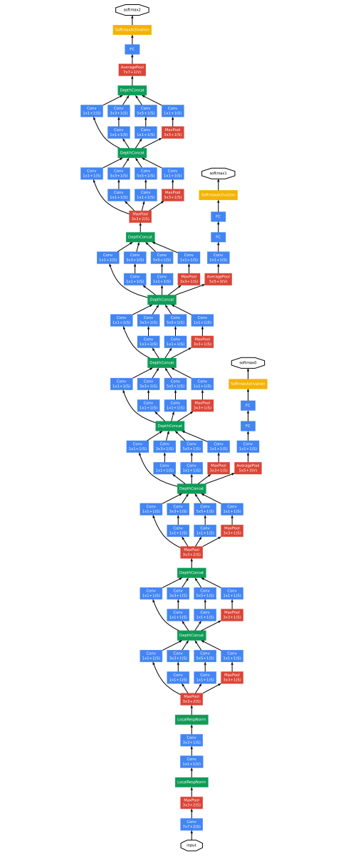
Figure 2: GoogleNet Convolutional Neural Network
Caffe Framework
Caffe is a deep learning framework made with expression, speed, and modularity in mind. It is developed by Berkeley AI Research (BAIR) and by community contributors. Yangqing Jia created the project during his PhD at UC Berkeley. Caffe is released under the BSD 2-Clause license.
Deep networks are compositional models that are naturally represented as a collection of inter-connected layers that work on chunks of data. Caffe defines a net layer-by-layer in its own model schema. The network defines the entire model bottom-to-top from input data to loss. As data and derivatives flow through the network in the forward and backward passes Caffe stores, communicates, and manipulates the information as blobs: the blob is the standard array and unified memory interface for the framework. The layer comes next as the foundation of both model and computation. The net follows as the collection and connection of layers. The details of blob describe how information is stored and communicated in and across layers and nets.
Implementation
The model used in this project is the GoogleNet neural network, whose parameters and weights were obtained after training step. The training phase is show in the Figure 3. This training is performed usig the Caffe framework. The design and layers of the GoogleNet networs is described in the
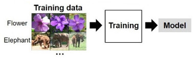
Figure 3: Training phase
After training step, the

Figure 4: Inference phase
As mentioned above, the pre-trained GoogleNet deep learning neural network is used in the Raspberry Pi to classify input images. However, when using the Raspberry Pi for deep learning we have two major pitfalls working against us:
- Restricted memory (only 1GB on the Raspberry Pi 3).
- Limited processor speed (four ARM Cortex-A53 core running at 1.2GHz on the Raspberry Pi 3).
This makes it difficult to use larger, deeper neural networks on this platform.
Despite these pitfalls, the Googlenet was implemented on the Raspberry Pi but taking certain considerations. Since the GoogleNet demands a high computational power, the time used by the Raspberry Pi to perform classification for each image is not enough to be processed in real time. So, instead to perform this classification in real time a single image will be captured by Pi Camera everytime a specific key is pushed.
The stream video is obtained using the Pi Camera module and using the Raspicam library. Then, the Raspberry Pi platforms classification using the GogoleNet pre-trained model. This classification for each image captured is realized using the deep neuronal libraries of OpenCV 3.3.0, which alllows the inference of pre-trained caffe models. In addition, this implementation was performed completely in C++.
The diagram of the recognition system is presented in the Figure 5:
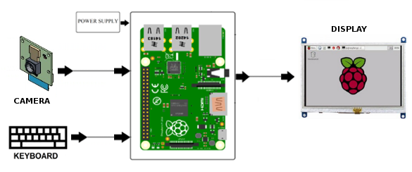
Figure 5: Diagram of the recognition system
Results
After the implementation of the GoogleNet model on the Raspberry Pi a series of objects were used for testing of the recognition system. The results obtained in this recognition system are shown in the Figure 6. These results show a high accuracy rate but a high processing time, which is about 3.4 seconds (average from 10 iterations).
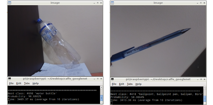
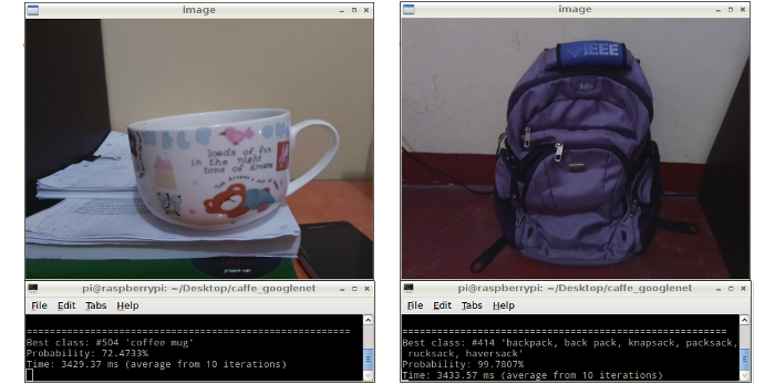
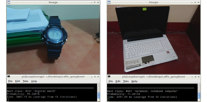
Figure 6: Results displayed in the LCD screen
Conclusions
In this project, the GoogleNet Deep Neural Network was implemented on a Raspberry Pi platform. The results show a high accuracy rate for different images. On the other hand, the time used to perform the image classification for each image is about 3.4 seconds (average from 10 iterations). This delay is because GoogleNet is composed by 22 layers (so, consider as a large deep neural network), which demands a high computational capacity for its processing.
Despite the long time used for classification, the GoogleNet was implemented succesfully with a high accuracy rate. In addition to this, future embedded hardware resources such as neuromorphic chips will allow the implementation of large neural networks in real time with a low energy consumption.